PLS on near-infrared spectra

Predicting a soil's organic carbon from its spectrum: the preprocessing, the number of components, the important variables, the validation, then new samples.

The data are simulated. No soil was measured: the spectra were made by the script spectres.R, with fixed seeds, from known absorption bands (organic matter, clay, water) and measurement defects (scatter, shifts, noise).

The question and the data

Measuring organic carbon in the laboratory is costly; measuring a near-infrared spectrum is cheap. With 120 samples that have both, can we predict the carbon of the next ones from their spectrum alone?

Download soils_spectra.csv (120 samples) and soils_new.csv (20 new ones, without their carbon):

Column	Content
sample	S001 to S120 (N001 to N020 for the new ones)
land_use	grassland or cropland
soc	the soil's organic carbon, in g/kg (not in the file of new samples)
1100 … 2500	the absorbance at each wavelength, from 1100 to 2500 nm every 10 nm (141 columns)

Open the first with File › Open: 120 observations and 143 variables. The columns named by a number are the variables of a spectrum, in the order of the table.

1. The model

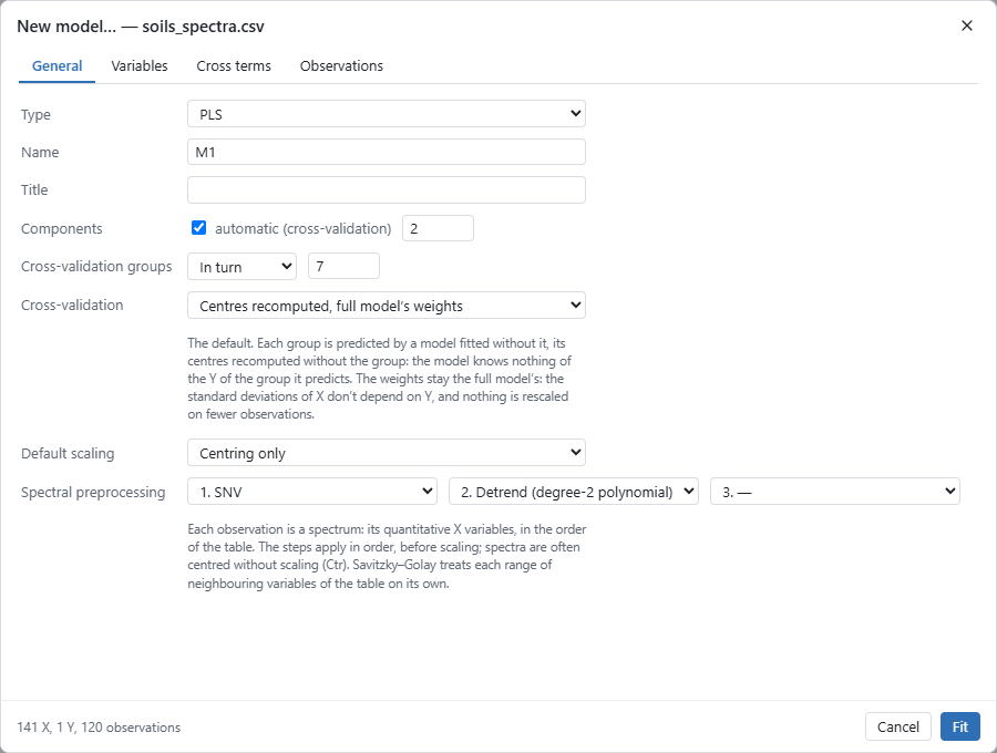
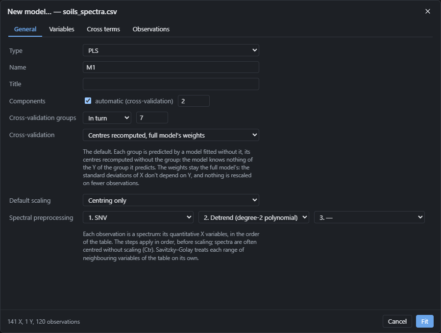
Model › New model (Ctrl+N). On the General tab:

Type: PLS;
Default scaling: Centring only. Spectra are often centred without scaling: the wavelengths keep their natural weight;
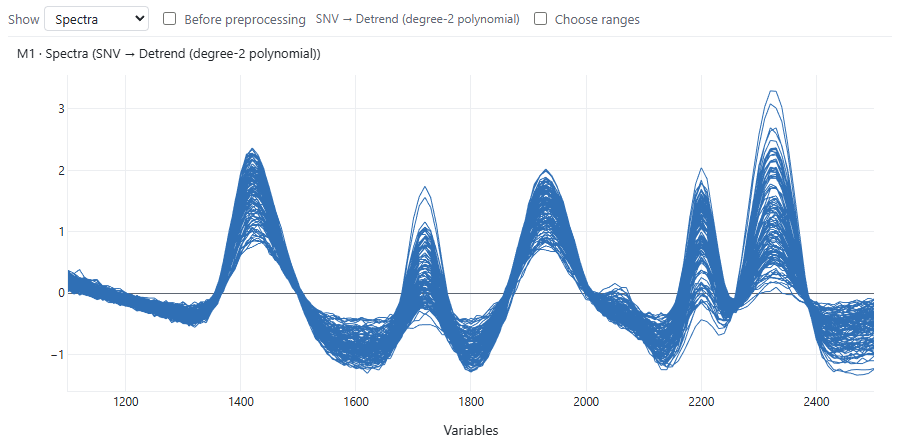
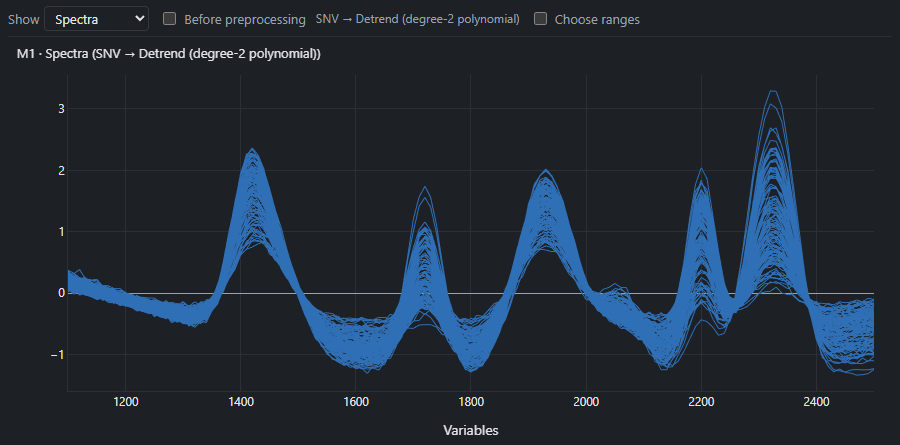
Spectral preprocessing: 1. SNV, then 2. Detrend (degree-2 polynomial). SNV centres each spectrum and divides it by its standard deviation, which removes the effect of grain size and packing; detrending removes the slope that remains (Barnes et al., 1989);
Components: automatic (cross-validation), with 7 groups in turn.

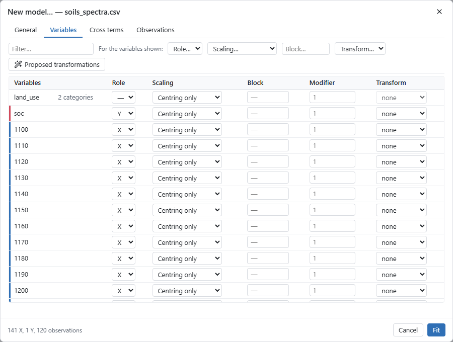
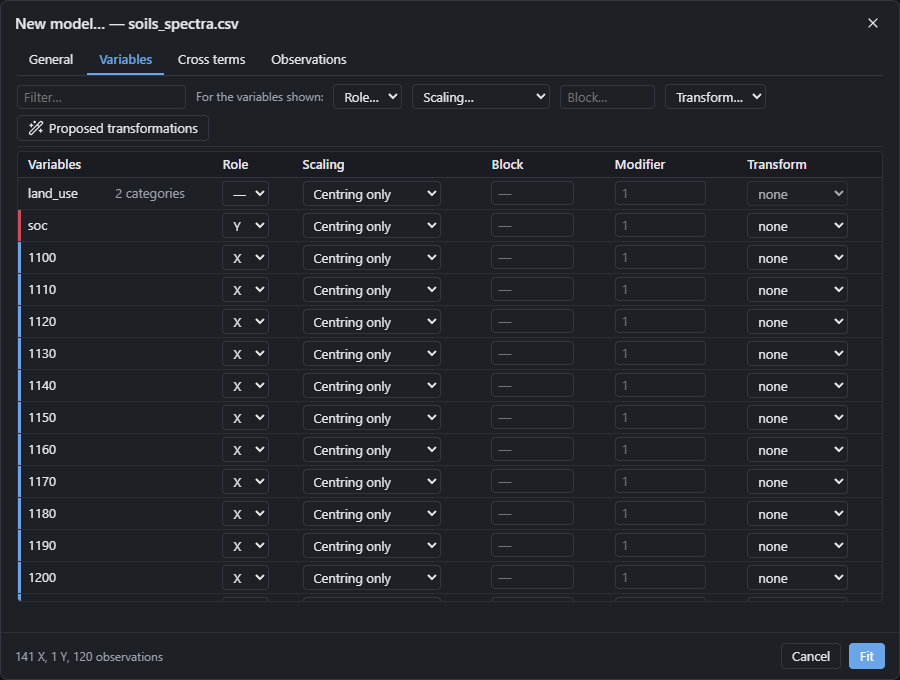
New model, General tab: PLS, centring only, SNV then detrend — The General tab: the type, the cross-validation, the scaling and the spectral preprocessing.

On the Variables tab, the Role… list above the table sets every variable shown at once: choose X, then give soc the role Y and leave land_use without a role (—).

New model, Variables tab: the wavelengths as X, soc as Y, land_use without a role — The Variables tab: 141 X, 1 Y, 120 observations.

Click Fit.

2. The spectra before and after preprocessing

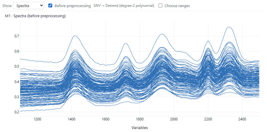
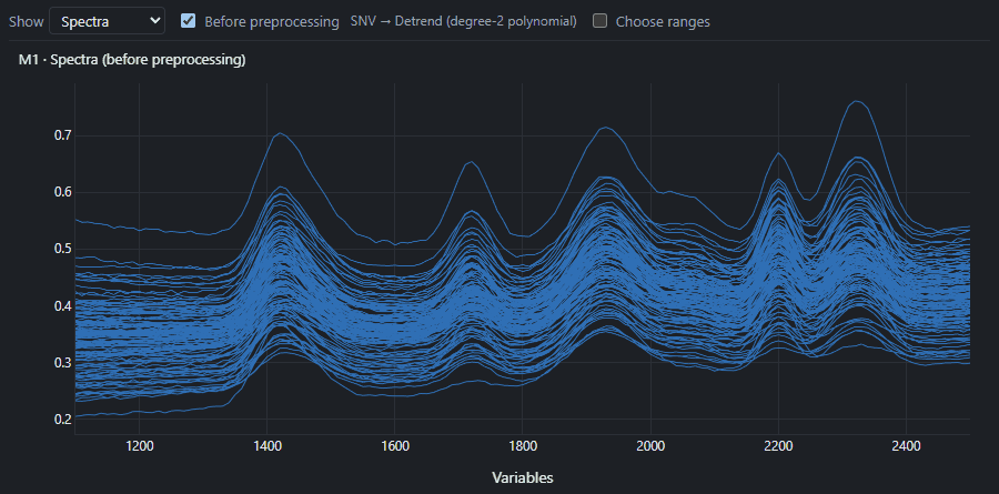
Plots › Profiles (spectra), Show: Spectra. Tick Before preprocessing to see the spectra as they were read: they are shifted and tilted against each other, and these differences have nothing to do with the carbon.

The 120 raw spectra, from 1100 to 2500 nm — Before preprocessing: the bands of water (1450, 1930 nm), clay (2200 nm) and organic matter (1720, 2310 nm), under shifts that vary from one sample to the next.

The same spectra after SNV and detrending — After SNV and detrending: the shifts are gone, the bands remain.

3. The Summary: how many components?

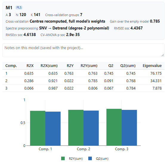
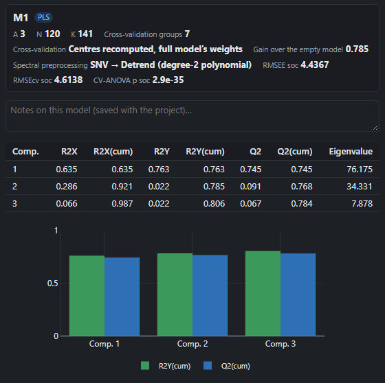
The PLS Summary: 3 components, R2X, R2Y and Q2 per component — The Summary: each component with the share of X and Y it explains and its Q2.

Autofit keeps 3 components: each improves the prediction in cross-validation (the component's Q2 is positive). Together they explain 98.7% of the spectra's variance (R2X) and 80.6% of the carbon's (R2Y). The cumulative Q2, the share of the carbon's variance predicted for samples the model hasn't seen, is 0.78.

In cross-validation, each group of samples is predicted by a model fitted without it: the prediction error (RMSEcv) is 4.6 g/kg, hardly more than the fitting error (RMSEE, 4.4 g/kg). The gain over the empty model (0.78) compares the model with the simplest prediction, the mean carbon. CV-ANOVA gives p < 0.001.

4. The important wavelengths

Plots › Profiles (spectra), Show: VIP. For a spectrum, VIP read better as a line against the wavelength.

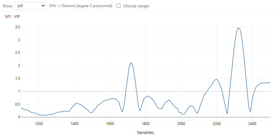
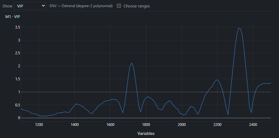
The model's VIP against the wavelength, with the line at 1 — The VIP: above 1, the wavelengths that count most to predict the carbon.

The highest VIP are around 2310 to 2350 nm and 1720 nm, two bands of organic matter (C–H bonds); lower, a clay band near 2200 nm and the end of the spectrum. The model does rely on the carbon's bands. Plots › VIP gives them as bars too, with a cut-off placed automatically; Refit with VIP variables makes the model again with those alone.

5. Observed and predicted

Plots › Observed vs predicted, coloured by land_use:

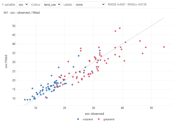
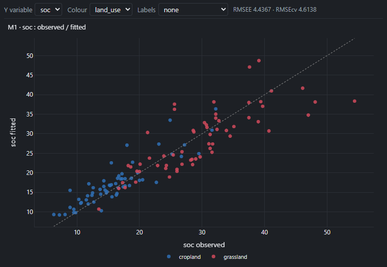
The carbon fitted by the model against the observed carbon, grasslands and croplands in colour — Observed against predicted: the points follow the diagonal; grasslands have more carbon than croplands.

The points follow the diagonal, grasslands at the top, croplands at the bottom. The richest soils (beyond 40 g/kg) are a little underestimated: there are few of them, and the model is linear.

6. The permutation test

A model of 141 variables for 120 observations can fit by chance. Plots › Permutation test shuffles the values of soc among the samples, refits the whole model, cross-validation included, and starts again (100 times here, 20 by default).

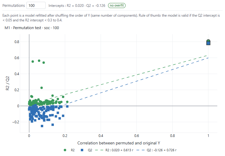
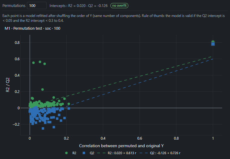
The permutation test: R2 and Q2 of the 100 permuted models against the correlation between the permuted and the original Y — The permutation test: on the left, the models fitted to a shuffled Y; on the right, the real model.

The models on a shuffled carbon have an R2 near 0 and a negative Q2: the lines' intercepts, R2 = 0.02 and Q2 = −0.13, are below the usual thresholds (0.3 to 0.4 for R2, 0.05 for Q2). The model doesn't come from overfitting.

7. Predicting new samples

Predict › Predict a file: choose soils_new.csv. Its columns are matched by their names; each spectrum is preprocessed like the model's, then projected onto its components.

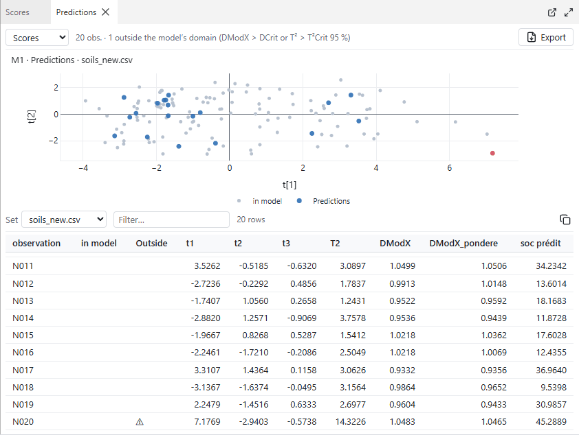
The predictions of the 20 new samples: their scores among the model's, and the table with the predicted carbon — The predictions: N020, in red, is outside the model's domain.

The last column gives each sample's predicted carbon. Nuée also flags those outside the model's domain, far from the calibration samples (T² beyond its 95% limit) or poorly described by the model (DModX beyond DCrit): here N020, far to the right on the scores plot. It is a peat soil, much richer in carbon than any calibration soil: its prediction (45 g/kg) is an extrapolation, and worth nothing. Such a sample is measured in the laboratory, and can then join the calibration. Export writes the table.

8. The Methods text

Model › Text for the Methods section writes, among other things:

Each spectrum (the 141 quantitative X variables, in table order) was first corrected by SNV (Barnes et al., 1989) and detrending (degree-2 polynomial removed; Barnes et al., 1989). The X variables were mean-centred only.

We fitted a PLS regression (partial least squares; Wold et al., 2001) with the NIPALS algorithm, with 3 components. Cross-validation used 7 groups (observation i in group i modulo 7); each group was predicted by a model fitted without it, with centring recomputed on the other observations and the scaling of the full model.

and the Results text gives the most important variables:

The most important variables (VIP > 1): 2320 (3.5), 2330 (3.4), 2310 (3.3), 2340 (3.2), 2300 (2.8), 2350 (2.6), 2290 (2.1), 1720 (2.1), among others.

Going further

Plots › iPLS (spectrum intervals) fits a PLS on each range of the spectrum and shows which predict best; Choose ranges, in the profiles view, makes a new model without a range (the water bands, for instance).
A test set (New model › Observations, at random or by Kennard–Stone) keeps samples out of the model and of the cross-validation, then predicts them.
File › Export to R writes a script that redoes the preprocessing, the NIPALS algorithm, the cross-validation and the plots in R alone, without any package.
The guide: spectra and their preprocessing, VIP, validation, cross-validation, the test set and prediction.