Before-after with controls (BACI)

Did removing a weir raise the density of young trout? A before-after control-impact design, from the table to the Methods text and the R script.

The data are simulated. No fish was counted: the table was made by the script baci.R, with a fixed seed, for this tutorial. It holds a known effect: +6 juveniles per 100 m² at the restored stations from 2016 on.

The question and the data

A mill weir was removed in the winter of 2015-2016. Every summer from 2010 to 2023, the year's juvenile trout are counted by electrofishing on six stations: three upstream of the former weir (A1, A2, A3: the impact) and three on a neighbouring tributary without a weir (T1, T2, T3: the controls). The controls follow the changes from one year to the next (floods, dry summers) that the restoration doesn't explain: the gap between impact and controls, before and after, measures its effect.

Download baci_trout.csv (84 rows, one per station and year):

Column	Content
obs	the row's name: the station and the year (A1-2010)
station	A1, A2, A3 (upstream of the weir), T1, T2, T3 (control tributary)
group	impact or control
year	2010 to 2023
density	juveniles per 100 m²; empty when the station wasn't fished (T2 in 2013, A3 in 2019)

Open it with File › Open (Ctrl+O): the project has 84 observations and 4 variables (the first column names the observations).

1. Which analysis?

Model › Which analysis?: tick Before-after with controls (BACI), then choose the response, density. Nuée proposes the time (year) and the unit (station) from their names, and recommends the before-after analysis with controls.

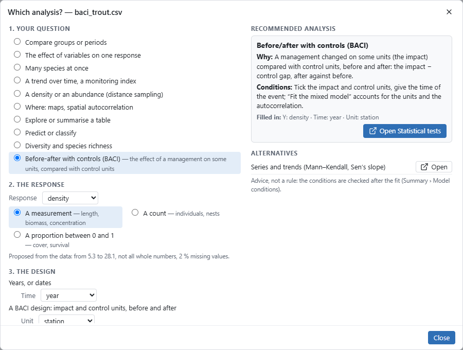
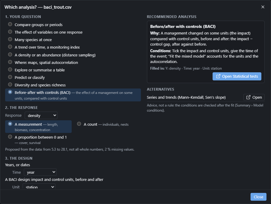
Which analysis? with the BACI question, the response density, the time and unit proposed, and the recommended analysis on the right — Which analysis?: the question, the response and the design on the left; the recommended analysis, its conditions and what is already filled in on the right.

Click Open Statistical tests: the tests view opens in its Before/after (BACI) mode, the response, the time and the unit already chosen.

2. The gap between impact and controls

Tick A1, A2 and A3 on the Impact line, then all the others on the Controls line. Type the year of the first "after" in Event: 2016.

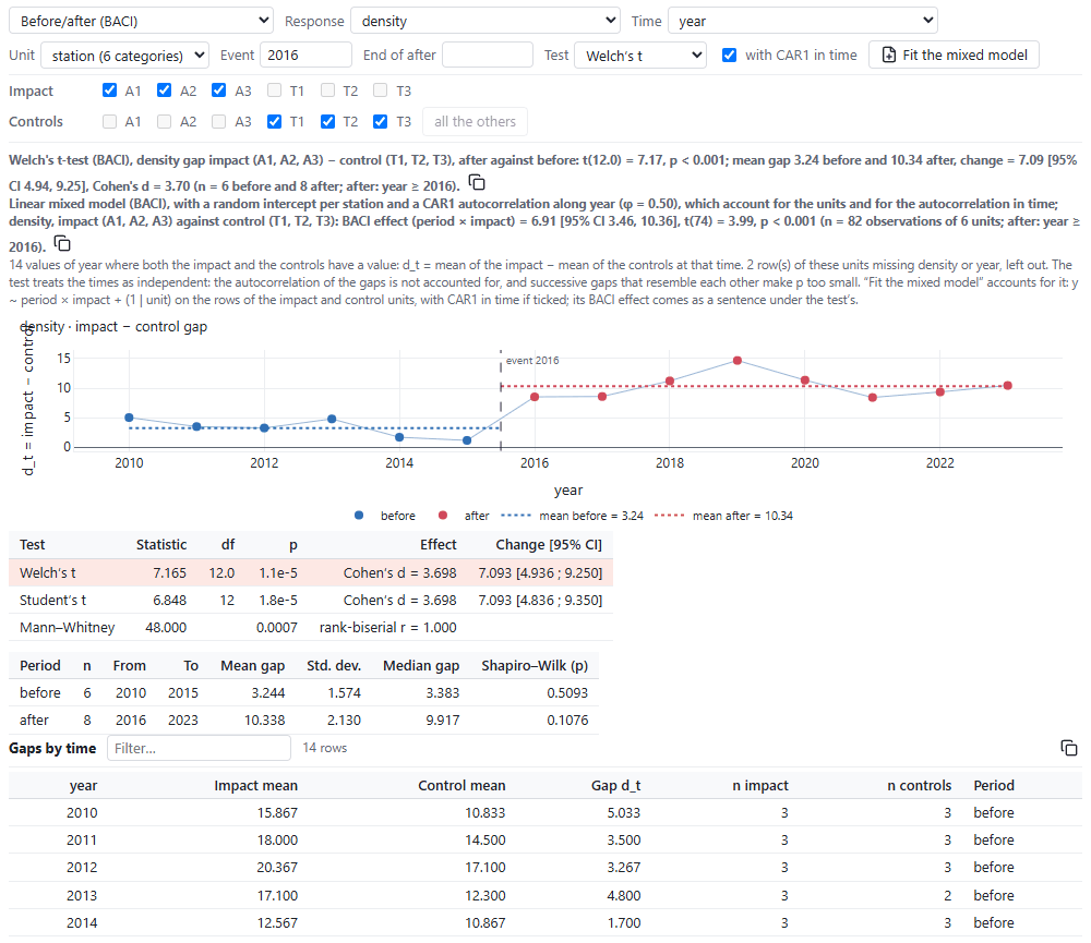
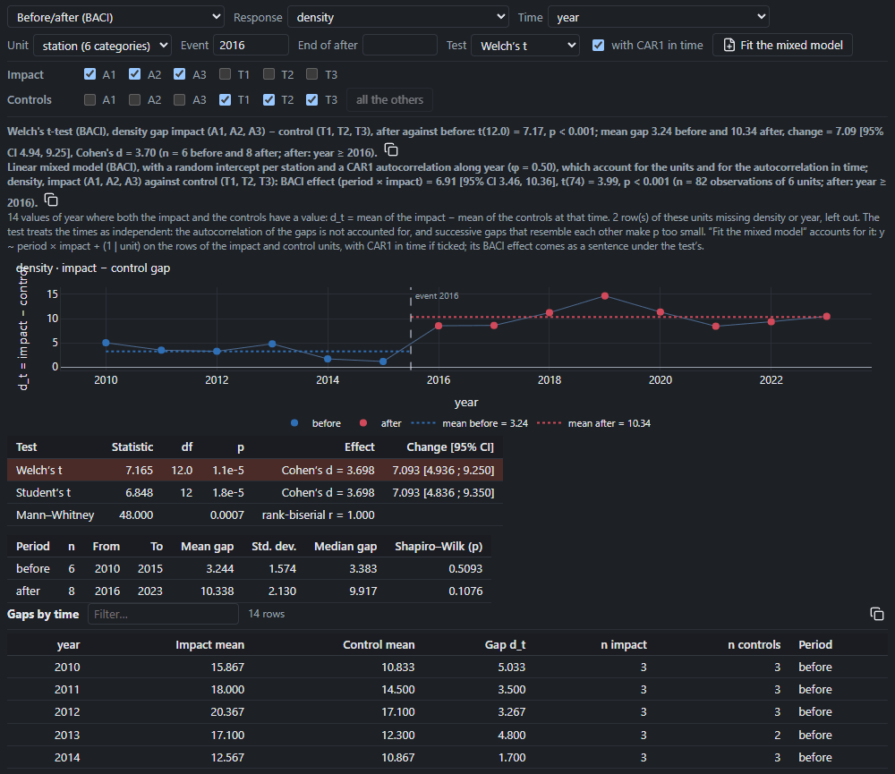
The BACI view: the stations ticked, the event 2016, the test's sentence and the plot of the impact − control gaps by year — The BACI view: each point is the gap between the mean of the impact stations and that of the controls in a year; the dotted lines, each period's mean.

Each year, the gap d_t is the mean of the impact stations minus that of the controls. Before the removal, the mean gap is 3.24 juveniles per 100 m²; after, 10.34. Welch's test compares the gaps after with those before: the change is 7.09 [95% CI 4.94, 9.25], p < 0.001.

This test takes the years as independent. But successive gaps often resemble each other (a good year follows a good one): the note under the sentence says so, and then p is too small. The mixed model accounts for it.

3. The BACI mixed model

With CAR1 in time is ticked (each station has at least three years). Click Fit the mixed model. Nuée adds to the project two variables worth 0 or 1:

"BACI period (2016)": 1 from 2016 on, 0 before;
"BACI impact (A1, A2, A3 vs T1, T2, T3)": 1 for the impact stations, 0 for the controls;

then fits the linear mixed model density ~ period × impact + (1 | station), with a random intercept per station and a CAR1 autocorrelation along the years within each station. The model is named "BACI density"; its views open. Back in the BACI view, its effect comes as a sentence under the test's (see the picture above): 6.91 [95% CI 3.46, 10.36], t(74) = 3.99, p < 0.001, with φ = 0.50.

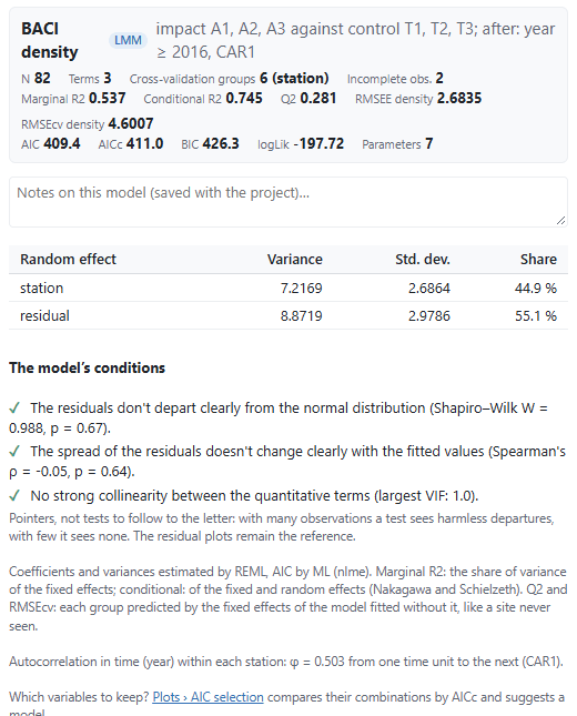
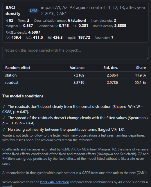
The BACI model's Summary: N, marginal and conditional R², Q², AIC, the variances of the random effects and the model conditions — The model's Summary: its quality, its random effects and its conditions, in words.

The Summary reads from top to bottom:

82 observations (2 without a density left out);
marginal R² 0.54 (the share of variance of the fixed effects), conditional R² 0.74 (with the differences between stations);
Q² 0.28: cross-validation predicts each station by a model fitted without it, by its fixed effects only, as a station never seen. A new station's own level is unknown: this modest Q² says nothing about the BACI effect;
the station carries 45% of the variance, the rest is residual; φ = 0.50: the correlation from one year to the next within a station.

The model conditions are said in words, each ✓ or ⚠ with what to do. Here all three are fine: the residuals don't depart clearly from the normal distribution (Shapiro–Wilk p = 0.67), their spread doesn't change with the fitted values, and the terms aren't collinear. These are pointers: the residual plots (Plots › Residuals) remain the reference.

4. Reading the interaction

Plots › Coefficients:

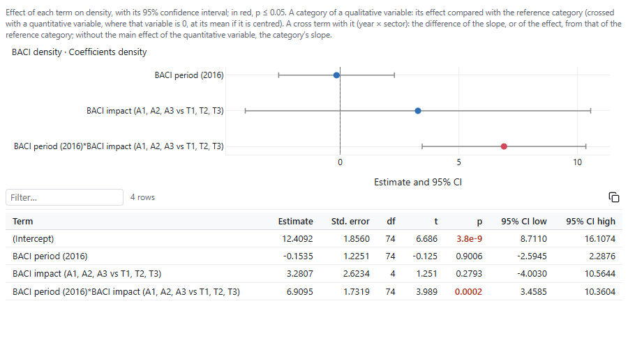
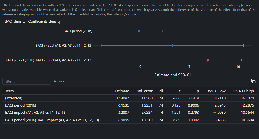
The coefficients of the BACI model: the period, the impact and their cross term, with their 95% intervals; the cross term in red — The coefficients: only the period × impact cross term is significant (in red).

The two variables being worth 0 or 1, each coefficient has a precise meaning:

Term	Estimate [95% CI]	What it measures
BACI period (2016)	−0.15 [−2.59, 2.29]	the change in the controls after 2016
BACI impact	3.28 [−4.00, 10.56]	the impact − control gap before 2016
period × impact	6.91 [3.46, 10.36]	the BACI effect: how much more the impact stations changed than the controls

The restoration's effect is the cross term, not the period's or the impact's coefficient taken alone. The upstream stations already had 3.3 more juveniles than the controls before the works (a gap that isn't significant, estimated with 4 degrees of freedom: it compares stations); comparing impact and controls after the works only would have counted that gap as an effect. The cross term compares each station with itself (74 degrees of freedom). The data were simulated with an effect of +6: the model estimates it at 6.9.

5. Adjusted means

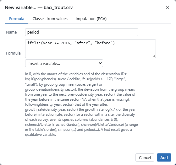
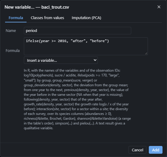
Adjusted means need qualitative variables. Make the period with Edit › New variable: name period, formula ifelse(year >= 2016, "after", "before") (a text result gives a qualitative variable).

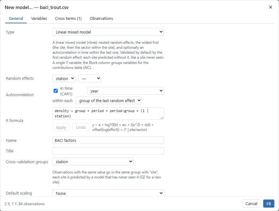
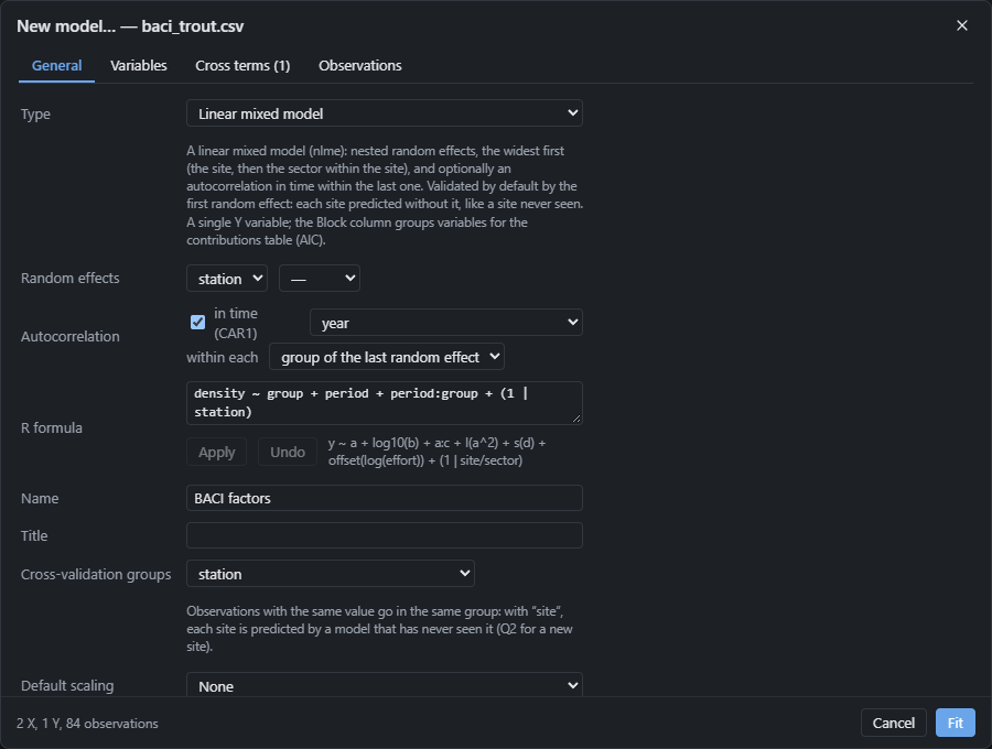
The New variable window, with the name period and its formula — New variable: an R formula on the other variables.

Then Model › New model: type Linear mixed model, and in R formula density ~ period * group + (1 | station), then Apply: the response, the two variables, their cross term and the station's random effect are set. Tick in time (CAR1) and choose year. Name it "BACI factors" and fit it: it is the same model, written with categories.

New model: linear mixed model, random effect station, CAR1 along year, the R formula applied — The same model, with the period and the group as qualitative variables.

Plots › Adjusted means: categories of period, within each level of group.

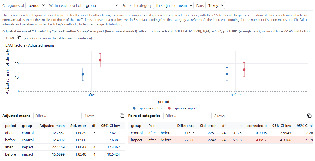
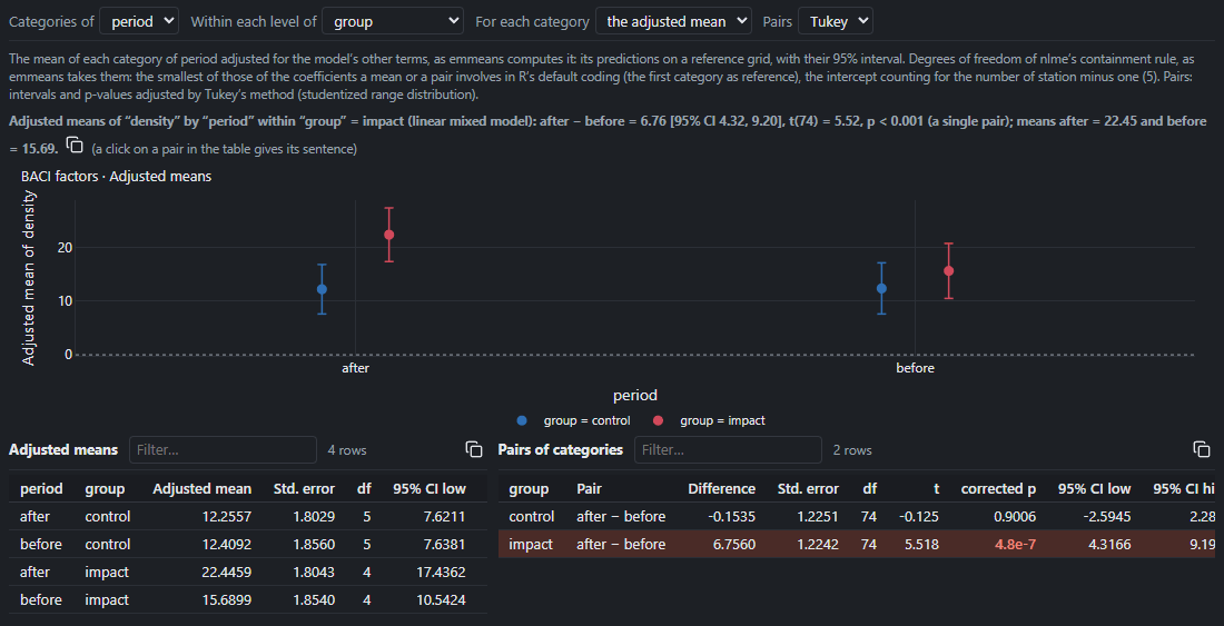
The adjusted means of density by period within each group, and the after − before pairs — The adjusted means: after against before, in the impact group and in the control group.

In the impact group, the density goes from 15.7 to 22.4 juveniles per 100 m²: +6.76 [95% CI 4.32, 9.20]. In the controls, from 12.4 to 12.3: −0.15 [−2.59, 2.29]. The difference between these two changes, 6.76 − (−0.15) = 6.91, is the BACI effect of the coefficient. A click on a pair of the table gives its sentence, to copy into a report.

6. The Methods and Results texts

Choose the "BACI density" model in the explorer, then Model › Text for the Methods section: a paragraph written from the model, in English or French, with its references, then the Results text.

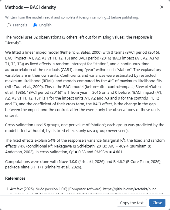
The Methods text of the BACI model, with the choice Français or English — The Methods text: to read over and complete before publishing.

It says, among other things:

This is the BACI model (before-after control-impact; Stewart-Oaten et al., 1986): “BACI period (2016)” is 1 from year = 2016 on and 0 before, “BACI impact (A1, A2, A3 vs T1, T2, T3)” is 1 for the impact units A1, A2 and A3 and 0 for the controls T1, T2 and T3, and the coefficient of their cross term, the BACI effect, is the change in the gap between the impact and the controls after the event; only the observations of these units enter it.

and for the results:

Coefficients (on the link scale): “BACI period (2016)”: β = -0.153 (95% CI [-2.59, 2.29], p = 0.9); “BACI impact (A1, A2, A3 vs T1, T2, T3)”: β = 3.28 (95% CI [-4.00, 10.6], p = 0.28); “BACI period (2016)*BACI impact (A1, A2, A3 vs T1, T2, T3)”: β = 6.91 (95% CI [3.46, 10.4], p < 0.001).

Complete it with what the model doesn't know: the fishing protocol, the area fished, the dates. Copy the text puts it on the clipboard.

7. Export to R

File › Export to R writes a script that refits the model without Nuée, with R and its nlme package (which comes with R): the data, the calculation written for this model (the fit by nlme::lme() with nlme::corCAR1(form = ~ year | station), the cross-validation by station, the statistics), then the tables and plots, all commented (about 250 lines here). As R Markdown or Quarto, it becomes a report with the Methods text.

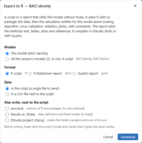
The Export to R window: this model or all those of the session, the format, the data in the script or in a CSV, and the files to write beside it — Export to R: a script for a colleague, or to attach to a paper.

Before writing, Nuée refits the model with the script and checks that it gives the same results. In the desktop application the button reads Choose where…; the screenshot comes from the browser version, where it downloads the files.

Going further

Plots › Residual autocorrelation shows the autocorrelation left from one year to the next; the models with and without CAR1 compare by AIC (Predict › Compare models).
The guide: statistical tests and the BACI mode, mixed models, their conditions and adjusted means, Export to R.